“Provide Python code examples for building a predictive maintenance model in Azure Machine Learning that connects to IoT data from factory equipment.”
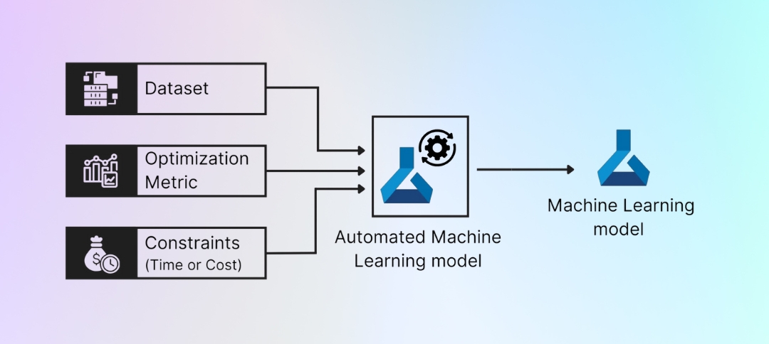
An effective predictive maintenance program for industrial equipment can be built by leveraging the Microsoft Azure ecosystem to ingest, process, and analyze Industrial Internet of Things (IIoT) data. By using Azure Machine Learning (Azure ML) with Python, you can create a robust solution that automates the entire process, from data preparation to model deployment. This approach shifts maintenance from a reactive or scheduled approach to a proactive, data-driven strategy, minimizing downtime and increasing operational efficiency.
An effective predictive maintenance program for industrial equipment can be built by leveraging the Microsoft Azure ecosystem to ingest, process, and analyze Industrial Internet of Things (IIoT) data. By using Azure Machine Learning (Azure ML) with Python, you can create a robust solution that automates the entire process, from data preparation to model deployment. This approach shifts maintenance from a reactive or scheduled approach to a proactive, data-driven strategy, minimizing downtime and increasing operational efficiency.

The Predictive Maintenance Workflow
The predictive maintenance process involves several key stages:
- Data Ingestion: Collect time-series sensor data (e.g., temperature, pressure, vibration) from factory machines.
- Data Preparation & Feature Engineering: Transform raw, granular data into meaningful features that represent a machine’s health over a specific time period. This is often the most critical step.
- Model Training: Use historical data with known failure events to train a classification model that predicts the likelihood of future failure.
- Model Deployment: Deploy the trained model as a REST API endpoint for real-time inference on new, incoming data.
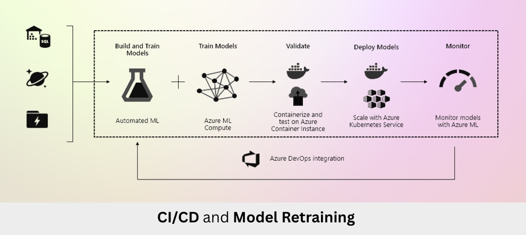
- Monitoring & Retraining: Continuously monitor the model’s performance and retrain it on new data to prevent model drift.
The following sections provide practical Python code examples for executing the first four steps within an Azure ML environment.
Prerequisites and Azure Setup
To follow this guide, you need:
- An Azure Subscription.
- An Azure Machine Learning Workspace: Create this via the Azure Portal or the Azure CLI.
- A Python Environment: Install the required libraries. Using an Azure ML Compute Instance is highly recommended as it comes pre-configured.
Bash
pip install azureml-core azureml-dataprep[pandas] scikit-learn pandas numpy joblib
Phase 1: Ingesting and Understanding the IoT Data
In a real-world scenario, data would stream from Azure IoT Hub into a datastore. For demonstration purposes, we will generate a synthetic dataset that mimics real-world sensor data, including anomalies that lead to a machine failure.
Python Code Example 1: Generating Synthetic IoT Sensor Data
This code generates time-series data for multiple machines. Each machine has a timestamp, a unique machine ID, and sensor readings for temperature, pressure, and vibration. Some simulated runs are configured to lead to a failure, marked by an error_code of 1.
Python
import pandas as pd
import numpy as np
from datetime import datetime, timedelta
def generate_synthetic_machine_data(machine_id, hours_of_operation, failure_occurred):
“””
Generates synthetic time-series data for a single machine.
“””
timestamps = [datetime.now() – timedelta(hours=hours_of_operation) + timedelta(minutes=x) for x in range(hours_of_operation*60)]
# Base values for sensors
base_temp = np.random.normal(50, 5)
base_pressure = np.random.normal(100, 10)
base_vibration = np.random.normal(10, 2)
data = {
‘timestamp’: timestamps,
‘machineID’: machine_id,
‘sensor_temperature’: [],
‘sensor_pressure’: [],
‘sensor_vibration’: [],
‘error_code’: 0 # Default to no error
}
failure_start_minute = hours_of_operation * 0.8 * 60 # Start anomaly at 80% of the timeline
for i, _ in enumerate(timestamps):
# Normal operation
temp = base_temp + np.random.normal(0, 1)
pressure = base_pressure + np.random.normal(0, 2)
vibration = base_vibration + np.random.normal(0, 0.5)
# Introduce a trend towards failure if applicable
if failure_occurred and i > failure_start_minute:
progression = (i – failure_start_minute) / (len(timestamps) – failure_start_minute)
temp += progression * np.random.normal(15, 3)
pressure += progression * np.random.normal(30, 5)
vibration += progression * np.random.normal(8, 1)
# Set error code in the final 5% of the failed run
if i > (len(timestamps) * 0.95):
data[‘error_code’] = 1
data[‘sensor_temperature’].append(temp)
data[‘sensor_pressure’].append(pressure)
data[‘sensor_vibration’].append(vibration)
return pd.DataFrame(data)
# Generate data for multiple machines and runs
all_machine_data = []
for machine_id in range(1, 6): # 5 machines
# Generate some normal runs and some failed runs
for _ in range(3): # 3 normal runs per machine
df = generate_synthetic_machine_data(f’M{machine_id}’, 120, failure_occurred=False)
all_machine_data.append(df)
for _ in range(1): # 1 failed run per machine
df = generate_synthetic_machine_data(f’M{machine_id}’, 120, failure_occurred=True)
all_machine_data.append(df)
final_df = pd.concat(all_machine_data, ignore_index=True)
print(final_df.head())
print(f”\nDataset shape: {final_df.shape}”)
print(f”Number of failure events (error_code=1): {final_df[‘error_code’].sum()}”)
This code creates a realistic time-series dataset where sensor readings gradually deviate from normal patterns before a failure event is flagged.
Phase 2: Feature Engineering for Time-Series Data
Raw minute-by-minute data is often too granular for a model to learn from effectively. We need to create features that capture the machine’s behavior over time windows (e.g., the last 1 hour, 6 hours). Rolling statistics are a common technique for this.
Python Code Example 2: Creating Rolling Features
This code calculates rolling averages, standard deviations, and rates of change for each sensor. It also creates the target label by shifting the error_code backward, creating a prediction window. This means the model will be trained to predict a failure in the next 12 hours.
Python
# Sort the data by machine and time
final_df.sort_values(by=[‘machineID’, ‘timestamp’], inplace=True)
features_list = []
# Group by machine to calculate features per machine
for machine_id, group in final_df.groupby(‘machineID’):
group = group.set_index(‘timestamp’)
# Calculate rolling features for each sensor
for sensor in [‘sensor_temperature’, ‘sensor_pressure’, ‘sensor_vibration’]:
# Rolling average and standard deviation over 1 hour (60 minutes)
group[f'{sensor}_mean_1h’] = group[sensor].rolling(window=’60min’, min_periods=1).mean()
group[f'{sensor}_std_1h’] = group[sensor].rolling(window=’60min’, min_periods=1).std()
# Rate of change (slope over the last 5 minutes)
group[f'{sensor}_slope’] = group[sensor].diff(periods=5) / 5
# Create the prediction label: 1 if failure occurs in the next 12 hours
prediction_window = ’12h’
group[‘label’] = (group[‘error_code’]
.rolling(window=prediction_window, min_periods=1)
.max()
.shift(periods=-(12*60), freq=’min’) # Shift backwards by 12 hours
).fillna(0) # Fill NA’s with 0 (no failure)
features_list.append(group)
# Combine the features back into one DataFrame
featured_df = pd.concat(features_list).reset_index()
# Drop rows with NA values caused by rolling calculations
featured_df.dropna(inplace=True)
print(featured_df[[‘timestamp’, ‘machineID’, ‘sensor_temperature_mean_1h’, ‘sensor_vibration_std_1h’, ‘label’]].head(10))

Phase 3: Training a Model in Azure Machine Learning
Now, we use Azure ML to train a model. This process involves creating an experiment, defining a compute target, and using the Python SDK to train a model and log its metrics.
Python Code Example 3: Azure ML Experimentation and Training
This script connects to the Azure ML workspace, registers the dataset, defines a compute cluster, trains a Random Forest Classifier with sklearn, and then logs the model and its metrics.
Python
from azureml.core import Workspace, Experiment, Dataset, Run
from azureml.core.compute import ComputeTarget, AmlCompute
from sklearn.model_selection import train_test_split
from sklearn.ensemble import RandomForestClassifier
from sklearn.metrics import accuracy_score, classification_report
import joblib
# Connect to your Azure ML Workspace
ws = Workspace.from_config() # Requires a config.json file from your workspace
# Register the featured dataset
datastore = ws.get_default_datastore()
registered_dataset = Dataset.Tabular.register_pandas_dataframe(
dataframe=featured_df,
target=datastore,
name=”predictive_maintenance_featured_data”,
description=”Synthetic IoT data with engineered features”
)
# Define a compute target (creates if it doesn’t exist)
compute_name = “cpu-cluster”
if compute_name not in ws.compute_targets:
compute_config = AmlCompute.provisioning_configuration(vm_size=’STANDARD_D2_V2′, max_nodes=4)
compute_target = ComputeTarget.create(ws, compute_name, compute_config)
compute_target.wait_for_completion(show_output=True)
else:
compute_target = ws.compute_targets[compute_name]
# Create an Azure ML experiment
experiment = Experiment(workspace=ws, name=’predictive-maintenance-experiment’)
# Start a run
with experiment.start_logging() as run:
# Load the data
df = registered_dataset.to_pandas_dataframe()
# Prepare data for training
feature_cols = [col for col in df.columns if ‘sensor_’ in col and (‘mean’ in col or ‘std’ in col or ‘slope’ in col)]
X = df[feature_cols]
y = df[‘label’].astype(int)
X_train, X_test, y_train, y_test = train_test_split(X, y, test_size=0.2, random_state=42, stratify=y)
# Train a model
model = RandomForestClassifier(n_estimators=100, random_state=42, class_weight=’balanced’)
model.fit(X_train, y_train)
# Evaluate the model
y_pred = model.predict(X_test)
accuracy = accuracy_score(y_test, y_pred)
# Log metrics and artifacts to Azure ML
run.log(“Accuracy”, accuracy)
run.log_list(“Feature Importances”, list(model.feature_importances_))
# Save the model
model_name = ‘predictive_maintenance_model.pkl’
joblib.dump(value=model, filename=model_name)
# Register the model in the Azure ML workspace
registered_model = run.register_model(model_name=’predictive-maintenance-rf’,
model_path=model_name,
description=’Random Forest model for equipment failure prediction’,
tags={‘area’: ‘IoT’, ‘type’: ‘classification’})
print(f”Model registered with accuracy: {accuracy:.4f}”)
print(classification_report(y_test, y_pred))
This script executes a full training run within Azure ML, automatically tracking all inputs, parameters, and outputs for complete reproducibility.
Phase 4: Deploying the Model for Real-Time Inference
The final step is to deploy the trained model as a web service. This allows new, incoming data to be sent to an endpoint, which then returns a real-time prediction.
Python Code Example 4: Creating a Scoring Script and Deploying
First, create the scoring script named score.py that will be used by the web service. It defines init() to load the model and run() to process incoming data and return a prediction.
Python
# File: score.py
import json
import joblib
import numpy as np
from azureml.core.model import Model
def init():
“””
This function is called when the container is initialized/started.
“””
global model
model_path = Model.get_model_path(‘predictive-maintenance-rf’)
model = joblib.load(model_path)
def run(raw_data):
“””
This function is called for every invocation of the endpoint.
“””
try:
data = json.loads(raw_data)[‘data’]
# The input data must be a list of lists or a 2D array
data_as_array = np.array(data)
# Get a prediction and probability from the model
prediction = model.predict(data_as_array).tolist()
proba = model.predict_proba(data_as_array).tolist()
return {“prediction”: prediction, “probability”: proba}
except Exception as e:
error = str(e)
return {“error”: error}
Next, in your main Python script, deploy the model using the score.py file.
Python
from azureml.core.webservice import AciWebservice, Webservice
from azureml.core.model import InferenceConfig, Model
from azureml.core.environment import Environment
# Connect to the workspace
ws = Workspace.from_config()
# Configure the inference environment with required packages
env = Environment(‘predictive-maintenance-env’)
env.python.conda_dependencies.add_pip_package(‘scikit-learn==1.0.2’) # Update scikit-learn version
env.python.conda_dependencies.add_pip_package(‘joblib==1.1.0’) # Update joblib version
env.python.conda_dependencies.add_pip_package(‘numpy==1.21.5’) # Update numpy version
env.python.conda_dependencies.add_pip_package(‘azureml-defaults’)
# Configure the inference configuration
inference_config = InferenceConfig(entry_script=’score.py’, environment=env)
# Configure the deployment target (Azure Container Instance is good for testing)
deployment_config = AciWebservice.deploy_configuration(cpu_cores=1, memory_gb=1)
# Get the registered model
model = Model(ws, ‘predictive-maintenance-rf’)
# Deploy the model
service = Model.deploy(workspace=ws,
name=’predictive-maintenance-service’,
models=[model],
inference_config=inference_config,
deployment_config=deployment_config,
overwrite=True)
service.wait_for_deployment(show_output=True)
print(f”Service state: {service.state}”)
print(f”Scoring URI: {service.scoring_uri}”)
Your predictive maintenance model is now live as a REST API. This endpoint can be integrated with Azure Stream Analytics or your factory’s IoT platform to provide real-time health assessments.
Conclusion: From Code to Operational Intelligence
This guide demonstrates how to build a scalable predictive maintenance solution using Python and Azure Machine Learning. By following these steps, from data synthesis and feature engineering to cloud-based model training and deployment, you can transform raw sensor data into actionable insights.
The true value of this approach lies in the seamless, managed MLOps lifecycle provided by Azure ML, which ensures your solution is reproducible and maintainable. This allows organizations to turn maintenance from a cost center into a strategic advantage powered by AI.
Recent Blogs